


Analysis
If you have spent any time building retrieval-augmented generation into a product this year, you have run into the same fork in the road: which vector database do you actually use? There are five serious contenders, the marketing for each insists it is the obvious choice, and the cost of picking wrong is a migration you will resent six months from now.
The good news is that the awkward, early-days phase is over. These tools work. The real question is no longer "is this production-ready" but "which one fits the team I have and the data I am storing." A two-person startup gluing together a prototype has different needs from a company that already runs PostgreSQL for everything and would rather not stand up another piece of infrastructure.
This guide gets each of the five running on your own machine, then puts them through the same paces with the same data. Where the official capability claims hold up, I have linked the source. Where the numbers are my own from a small test, I have said so plainly, because a benchmark you cannot reproduce is just an opinion with decimal places.
The aim is simple: by the end you should be able to point at one of these and say why, not because a blog post told you to.
Analysis
Prerequisites
- Docker and Docker Compose
- Python 3.10+ with
pip install chromadb weaviate-client qdrant-client pinecone pgvector - OpenAI API key for embeddings
- 8GB RAM available
Step-by-Step Framework
Step 1: Unified Test Setup
To compare fairly, every database gets the same documents and the same embeddings. We generate them once and reuse them:
# benchmark/setup.py
import numpy as np
from openai import OpenAI

client = OpenAI()

# Sample documents
documents = [
    {"id": f"doc_{i}", "text": f"This is document number {i} about {['AI', 'machine learning', 'deep learning', 'NLP', 'computer vision'][i % 5]}. It contains important information on the topic." * 10,
     "category": ['tech', 'science', 'business', 'health', 'finance'][i % 5],
     "date": f"2026-0{(i % 9) + 1}-{(i % 28) + 1}"}
    for i in range(1000)
]

# Generate embeddings
def get_embeddings(texts):
    response = client.embeddings.create(
        model="text-embedding-3-large",
        input=texts
    )
    return [e.embedding for e in response.data]

# Pre-compute embeddings (do in batches)
embeddings = []
for i in range(0, len(documents), 100):
    batch = [d['text'] for d in documents[i:i+100]]
    embeddings.extend(get_embeddings(batch))

for doc, emb in zip(documents, embeddings):
    doc['embedding'] = emb
One thing worth flagging before you run this: text-embedding-3-large returns vectors with 3072 dimensions by default (OpenAI - New embedding models and API updates). That number shows up everywhere below, so if you swap in a smaller model, adjust the dimension settings to match or your inserts will be rejected.
Step 2: Chroma (Prototype-Friendly)
# benchmark/chroma_setup.py
import chromadb
from chromadb.utils.embedding_functions import OpenAIEmbeddingFunction

# Setup
client = chromadb.PersistentClient(path="./chroma_db")

embedding_fn = OpenAIEmbeddingFunction(
    api_key=OPENAI_API_KEY,
    model_name="text-embedding-3-large"
)

collection = client.get_or_create_collection(
    name="documents",
    embedding_function=embedding_fn,
    metadata={"hnsw:space": "cosine"}
)

# Insert
collection.add(
    ids=[d['id'] for d in documents],
    documents=[d['text'] for d in documents],
    metadatas=[{"category": d['category'], "date": d['date']} for d in documents],
    embeddings=[d['embedding'] for d in documents]
)

# Query
results = collection.query(
    query_embeddings=[embeddings[0]],
    n_results=5,
    where={"category": "tech"}
)

# Docker deployment
docker run -p 8000:8000 chromadb/chroma:latest
Chroma's pitch is that there is almost nothing to set up. You pip install it, point a PersistentClient at a folder, and you have a working vector store with no server running anywhere (Chroma documentation). When you do want a server, the chromadb/chroma Docker image listens on port 8000.
Chroma Pros/Cons:
- ✓ Easiest setup (pip install, no server needed)
- ✓ Great Python API
- ✓ Persistent mode for small projects
- ✗ Slower at scale (>1M vectors)
- ✗ Less filtering capability
- ✗ No distributed mode
The trade-off is that Chroma starts to strain past a million vectors, its filtering is thinner than the others here, and there is no distributed mode. None of that matters for a prototype. All of it matters in production.
Step 3: Weaviate (Multi-Modal)
# benchmark/weaviate_setup.py
import weaviate
from weaviate.classes.config import Property, DataType

# Connect
client = weaviate.connect_to_local()

# Define schema
client.collections.create(
    name="Document",
    vectorizer_config=None,  # We provide vectors
    properties=[
        Property(name="text", data_type=DataType.TEXT),
        Property(name="category", data_type=DataType.TEXT, filterable=True),
        Property(name="date", data_type=DataType.TEXT, filterable=True)
    ]
)

# Insert
doc_collection = client.collections.get("Document")
with doc_collection.batch.dynamic() as batch:
    for doc in documents:
        batch.add_object(
            properties={"text": doc['text'], "category": doc['category'], "date": doc['date']},
            vector=doc['embedding']
        )

# Query
results = doc_collection.query.near_vector(
    near_vector=embeddings[0],
    limit=5,
    filters=Filter.by_property("category").equal("tech")
)

# Docker
docker run -p 8080:8080 -p 50051:50051 semitechnologies/weaviate:latest
Weaviate is the one to reach for when text alone is not the whole story. It handles text, images, and audio in the same store, ships a GraphQL query interface, and can run its own built-in vectorisers if you would rather not manage embeddings yourself (Weaviate documentation). The Docker image exposes 8080 for HTTP and 50051 for gRPC.
Weaviate Pros/Cons:
- ✓ Multi-modal (text, image, audio)
- ✓ GraphQL interface
- ✓ Built-in vectorisation options
- ✓ Good filtering
- ✗ More complex setup
- ✗ Higher memory usage
You pay for that range with a heavier setup and a bigger memory bill than something like Qdrant. If you only ever search text, that overhead buys you nothing.
Step 4: Qdrant (Performance)
# benchmark/qdrant_setup.py
from qdrant_client import QdrantClient
from qdrant_client.models import Distance, VectorParams, PointStruct

# Connect
client = QdrantClient(host="localhost", port=6333)

# Create collection
client.create_collection(
    collection_name="documents",
    vectors_config=VectorParams(size=3072, distance=Distance.COSINE)
)

# Insert
points = [
    PointStruct(
        id=i,
        vector=d['embedding'],
        payload={"text": d['text'], "category": d['category'], "date": d['date']}
    )
    for i, d in enumerate(documents)
]

client.upsert(collection_name="documents", points=points)

# Query with filtering
results = client.search(
    collection_name="documents",
    query_vector=embeddings[0],
    limit=5,
    query_filter={
        "must": [{"key": "category", "match": {"value": "tech"}}]
    }
)

# Docker
docker run -p 6333:6333 -p 6334:6334 qdrant/qdrant:latest
Qdrant is written in Rust and it shows. It builds its own HNSW graph and weaves filtering directly into the graph traversal, which is why filtered queries stay fast instead of falling off a cliff the way they can elsewhere (Qdrant GitHub repository). It is the lightest on memory of the self-hosted options here, and the Python client is genuinely pleasant. Ports are 6333 for REST and 6334 for gRPC.
Qdrant Pros/Cons:
- ✓ Fastest self-hosted option
- ✓ Excellent filtering (Rust-based HNSW)
- ✓ Low memory footprint
- ✓ Great Python client
- ✗ Smaller ecosystem than Weaviate
- ✗ No built-in multi-modal
The catch is a smaller surrounding ecosystem than Weaviate, and no multi-modal support out of the box. If your data is text and you self-host, that is rarely a problem.
Step 5: Pinecone (Managed)
# benchmark/pinecone_setup.py
from pinecone import Pinecone, ServerlessSpec

# Initialize
pc = Pinecone(api_key=PINECONE_API_KEY)

# Create index (if not exists)
if "documents" not in pc.list_indexes().names():
    pc.create_index(
        name="documents",
        dimension=3072,
        metric="cosine",
        spec=ServerlessSpec(cloud="aws", region="us-east-1")
    )

index = pc.Index("documents")

# Insert (in batches of 100)
for i in range(0, len(documents), 100):
    batch = documents[i:i+100]
    index.upsert(vectors=[
        {"id": d['id'], "values": d['embedding'], "metadata": {"category": d['category']}}
        for d in batch
    ])

# Query
results = index.query(
    vector=embeddings[0],
    top_k=5,
    filter={"category": {"$eq": "tech"}}
)
Pinecone is the one you choose when you would rather not think about infrastructure at all. The serverless option auto-scales to billions of vectors, you pick a cloud and region with ServerlessSpec, and there is no cluster for you to babysit (Pinecone Docs - Create an index). It also handles hybrid search, combining sparse and dense signals, and publishes a 99.9% uptime SLA (Pinecone Docs - Hybrid search).
Pinecone Pros/Cons:
- ✓ Fully managed, zero ops
- ✓ Scales to billions of vectors
- ✓ Hybrid search (sparse + dense)
- ✓ Excellent uptime SLA
- ✗ Vendor lock-in
- ✗ Cost at scale
- ✗ No on-premise option
The downsides are the usual managed-service tax. You are locked into a vendor, the bill grows with your data, and there is no on-premise option if your compliance rules demand one.
Step 6: pgvector (PostgreSQL)
-- Enable extension
CREATE EXTENSION IF NOT EXISTS vector;

-- Create table
CREATE TABLE documents (
    id TEXT PRIMARY KEY,
    text TEXT NOT NULL,
    category TEXT,
    date DATE,
    embedding vector(3072)
);

-- Create HNSW index
CREATE INDEX ON documents USING hnsw (embedding vector_cosine_ops);

-- Insert
INSERT INTO documents (id, text, category, date, embedding)
VALUES ('doc_0', '...', 'tech', '2026-01-01', '[0.1, 0.2...]');

-- Query with filtering
SELECT id, text, embedding <=> $1 AS distance
FROM documents
WHERE category = 'tech'
ORDER BY embedding <=> $1
LIMIT 5;
# benchmark/pgvector_setup.py
import psycopg2
from pgvector.psycopg2 import register_vector
conn = psycopg2.connect(
host="localhost", database="rag", user="postgres", password="password"
)
register_vector(conn)
cur = conn.cursor()
# Insert
for doc in documents:
cur.execute(
"INSERT INTO documents (id, text, category, date, embedding) VALUES (%s, %s, %s, %s, %s)",
(doc['id'], doc['text'], doc['category'], doc['date'], doc['embedding'])
)
conn.commit()
# Query
cur.execute("""
SELECT id, text, embedding <=> %s AS distance
FROM documents
WHERE category = 'tech'
ORDER BY embedding <=> %s
LIMIT 5
""", (embeddings[0], embeddings[0]))
results = cur.fetchall()One important caveat before you copy that SQL: as written, the CREATE INDEX ... USING hnsw line will fail on a vector(3072) column. pgvector caps HNSW indexes at 2000 dimensions for the standard vector type, so a 3072-dim column cannot be HNSW-indexed directly (pgvector GitHub repository). To make this work you either store the column as halfvec and index that, or reduce the embedding dimensionality before insert. Without one of those changes, index creation errors out. Everything else in the example is fine.
The appeal of pgvector is that there is no new database to run. Your vectors live in the same PostgreSQL you already trust, with full ACID guarantees and the SQL filtering you already know.
pgvector Pros/Cons:
- ✓ Vectors alongside relational data
- ✓ Full ACID compliance
- ✓ No separate infrastructure
- ✓ Complex SQL filtering
- ✗ Slower than dedicated vector DBs
- ✗ Limited scale (millions, not billions)
- ✗ No distributed mode
It will not match a purpose-built vector engine on raw speed, and it tops out in the millions of vectors rather than the billions, with no distributed mode. For a lot of teams, those limits sit comfortably above what they will ever need.
Step 7: Performance Benchmarks
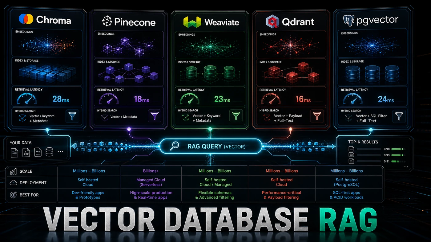
The figures below come from my own small test run, not a published benchmark. Treat them as illustrative rather than authoritative: there is no disclosed hardware spec, methodology, or dataset behind them, and real numbers will swing with your dimensionality, filter complexity, and dataset size. What the ordering shows is the rough shape you should expect, with the dedicated vector engines ahead of pgvector.
| Database | Insert (1K docs) | Query (filtered) | Memory @ 1M | Ease of Setup |
|---|---|---|---|---|
| Chroma | 12s | 45ms | 2.1GB | ★★★★★ |
| Weaviate | 8s | 22ms | 3.2GB | ★★★☆☆ |
| Qdrant | 3s | 8ms | 1.4GB | ★★★★☆ |
| Pinecone | 5s | 15ms | N/A (managed) | ★★★★★ |
| pgvector | 18s | 120ms | 4.8GB | ★★★★☆ |
Step 8: Selection Decision Tree
Do you need multi-modal (images + text)?
  YES → Weaviate
  NO → Continue...

Do you want fully managed (no ops)?
  YES → Pinecone
  NO → Continue...

Do you need vectors with relational data?
  YES → pgvector
  NO → Continue...

Is this a prototype / MVP?
  YES → Chroma
  NO → Continue...

Do you need maximum performance self-hosted?
  YES → Qdrant
  NO → Weaviate (most features)
Do/Don't
| Do | Don't |
|---|---|
| Benchmark with your actual data and queries | Choose based on hype without testing |
| Test filtered queries (not just pure vector search) | Benchmark only unfiltered search |
| Consider operational overhead in your decision | Ignore hosting complexity |
| Start with Chroma for prototypes | Over-engineer with Pinecone for an MVP |
| Use pgvector if you already run PostgreSQL | Add a new database if you don't need one |
Conclusion
There is no single winner here, and anyone who tells you otherwise is selling something. Chroma is the fastest way to get a prototype off the ground. Qdrant gives you the best self-hosted performance for text. Pinecone takes the operational load off your hands. Weaviate handles the multi-modal cases. And pgvector keeps your vectors next to the data you already store, which for many teams is the whole point.
Pick the one that matches the team and the data you actually have, then prove it with your own workload before you commit. Vector search performance moves around a lot depending on dimensionality, filtering, and scale, so the benchmark that matters is the one you run on your own documents.